Andrew L. and Andrew Z.
Computational Physics
Problem Statement
There are numerous (or innumerable) methods for modeling and considering characteristics of rocket trajectory. These models present advantages in simplicity or complexity depending on the intended model application. A trajectory model intended for a commercial customer may be exceptionally resource intensive in set-up cost or processing resources but may be necessary depending on the computational design basis’s accuracy, precision, and stability. A less process-intensive model may be simpler to compute and present less initial setup investment but may not meet the requirements for much beyond a theoretical application.
We intend to model rocket trajectories considering various computational models. We intend to compare variations in Deterministic and Probabilistic computational models for rocket trajectories and identify models that present value in processing efficiency, flexibility, and exhaustiveness in analysis.
The goal of our analysis it to develop a flexible computation model that could provide analytic value to characterize trajectory and drag of projectile motion in a wide range of environmental conditions.
Methods
We model the trajectory of a rocket that decreases in mass as it expends fuel, in a 3-dimensional, cartesian basis. This model considers rocket mass, gravity, and thrust, Additionally we generate atmospheric condition models to analyze the influence of atmospheric temperature, pressure, and density on drag resistance as well as this influence on elements of trajectory. The ideal rocket differential equation is our starting basis and we will add more factors to provide a realistic and complete model simulation.

Considering Drag

We use the force drag equation that depends on the density of air, rocket velocity, drag coefficient, and surface area. To incorporate this analysis into a Modified Euler, corresponding values of altitude, temperature, pressure, and density are necessary.
Atmosphere Modeling
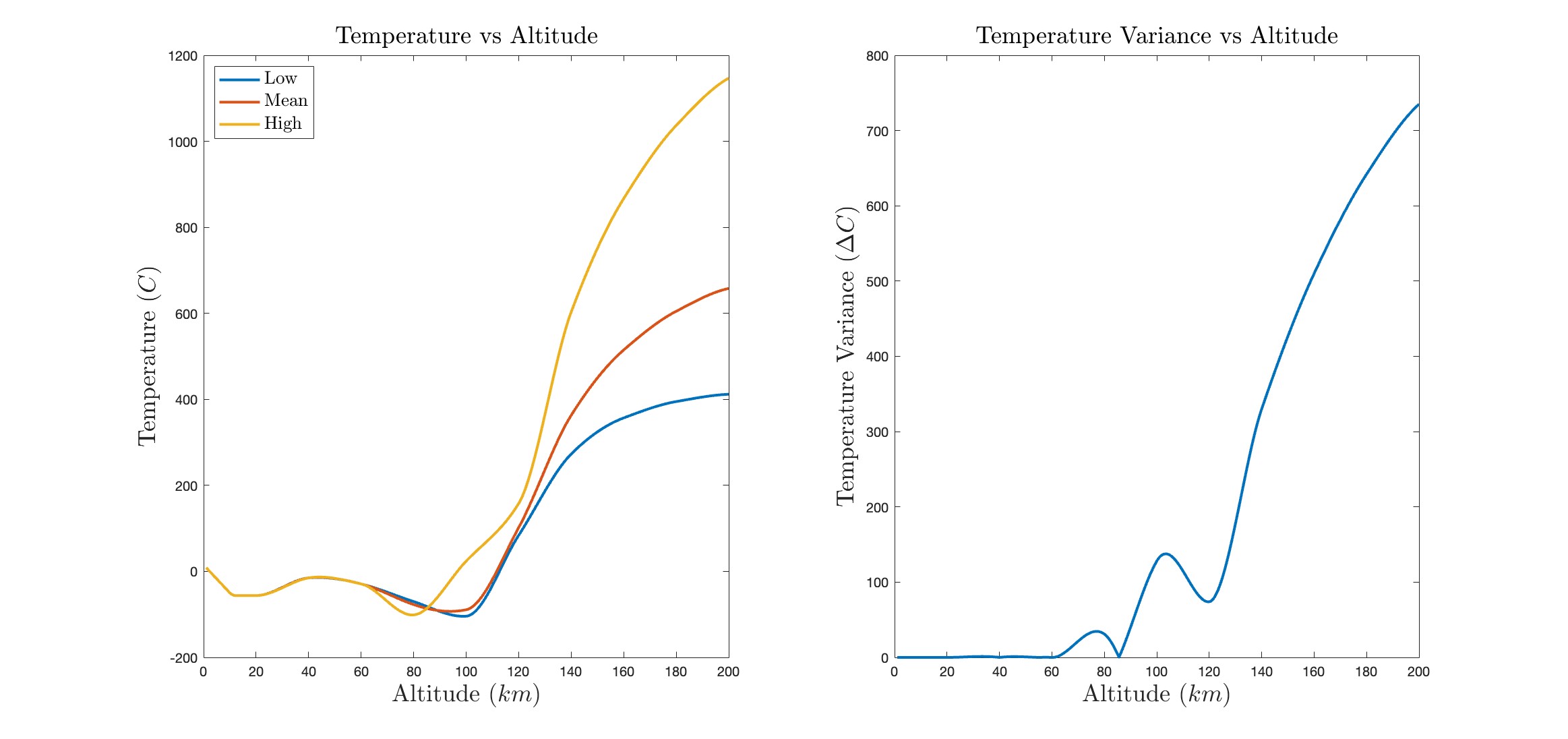
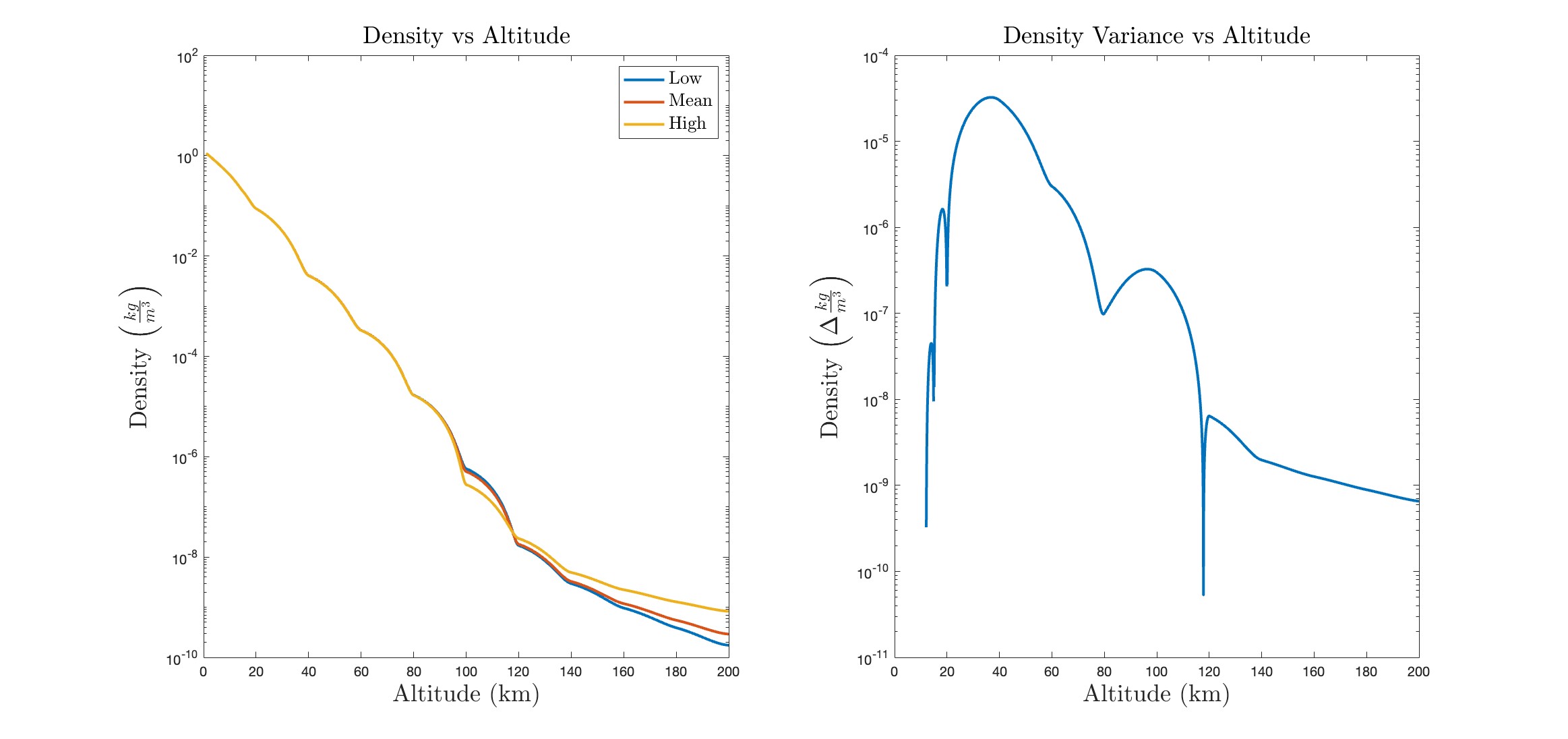
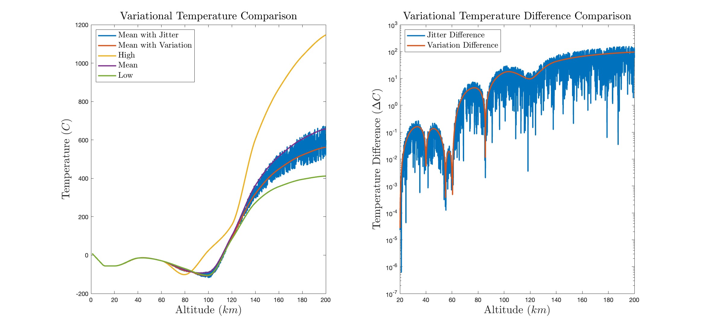
We use known values to generate a set of values for atmospheric temperature, pressure, and density as a function of altitude. For temperature, we derive values based on the observed temperature at altitudes during periods of low, mean, and high solar activity. We consider a combination of data values from Properties Of The U.S. Standard Atmosphere 1976 and the MSISE-90 Model of Earth’s Upper Atmosphere to generate a range of values with some variation in data throughout the atmospheric layers.1,2
Data Interpolation
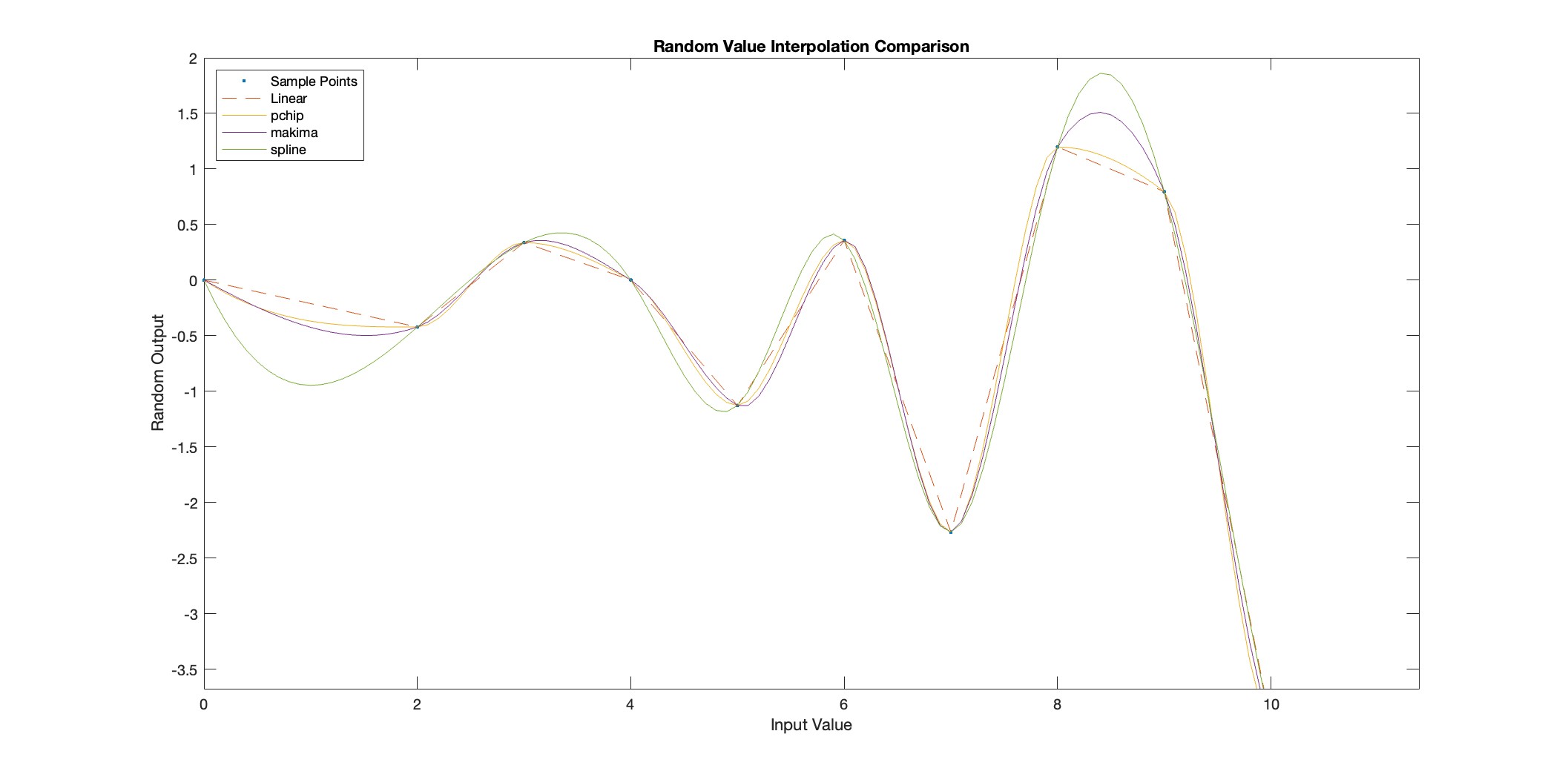
The data sets gather large amount of information about changes in characteristics throughout the atmosphere; however, the intervals between data values present discontinuities and incomplete information about rates of change and would be unsuitable for Modified Euler Methods. We use interpolation to obtain a continuous range of values with reasonable physical meaning. We consider linear interpolation, piecewise-cubic interpolation, cubic convolution, Modified Akima cubic Hermite interpolation, and spline interpolation.
Methods of interpolation vary in and computational efficiency. and depending on where this analysis is used in the model, efficiency could extend run times to make the code unusable with only marginal utility. Since we only generate an environmental model once, prior to calculating trajectory, efficiency is not a primary concern.
Temperature, Pressure, and Density Modeling
We model temperature based on the known values to at kilometers of altitude above earth surface to consider low-, mid-, and high- solar activity generate a range range of values. Temperature variance, due to solar activity, has a marginal influence below 60km altitude.
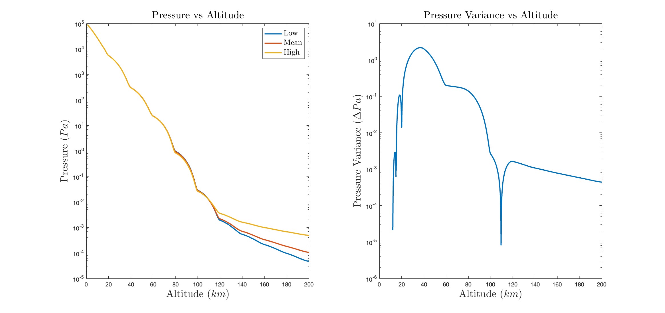
We model pressure and density based on the known values with similar consideration of solar activity.
Deterministic and Probabilistic Analysis
We add randomness to account for variations in atmospheric conditions. We initially use a range of values for reasonable atmospheric conditions and consider a standard proportional variation within this range.
In addition we consider a standard proportional variation with another random variation at every data point.
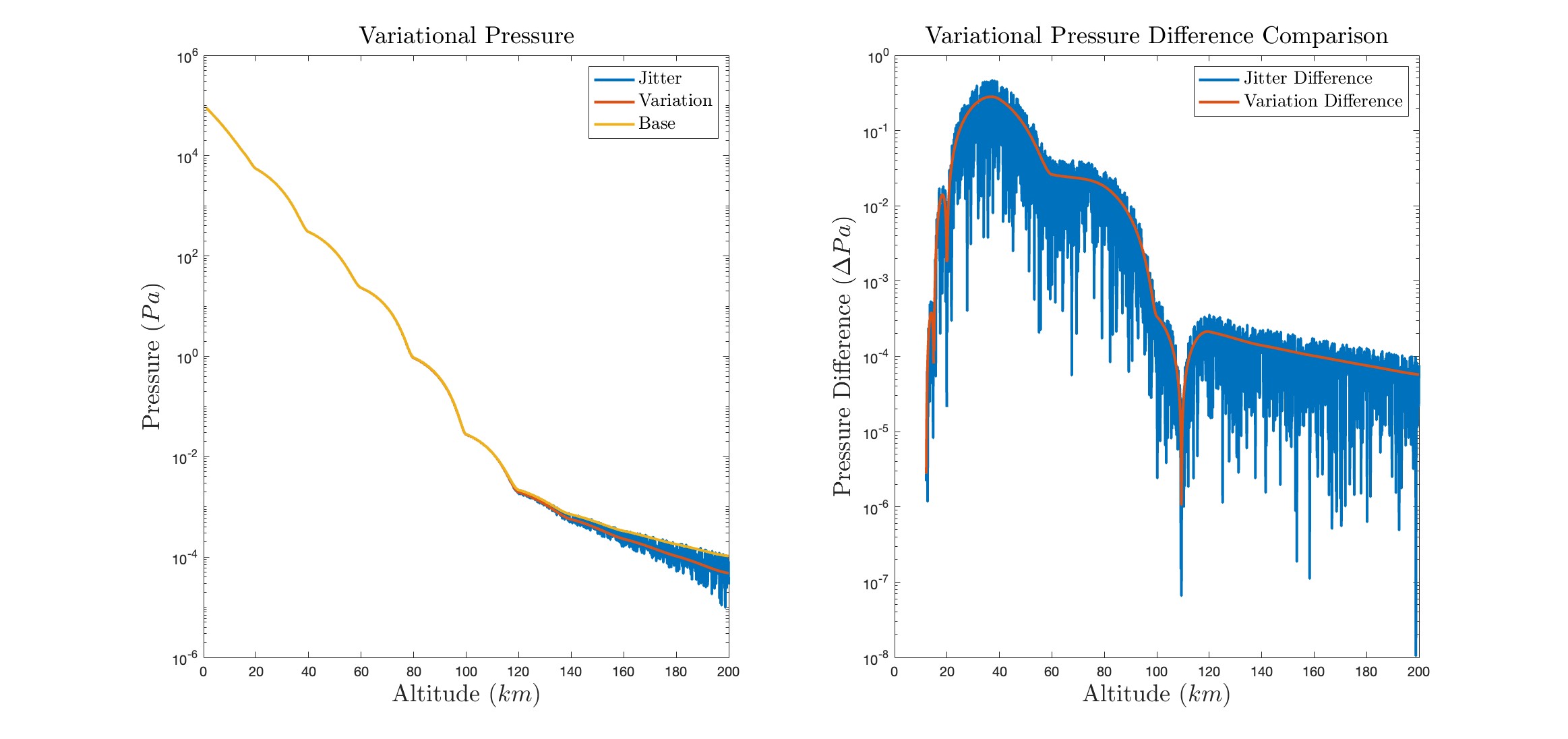
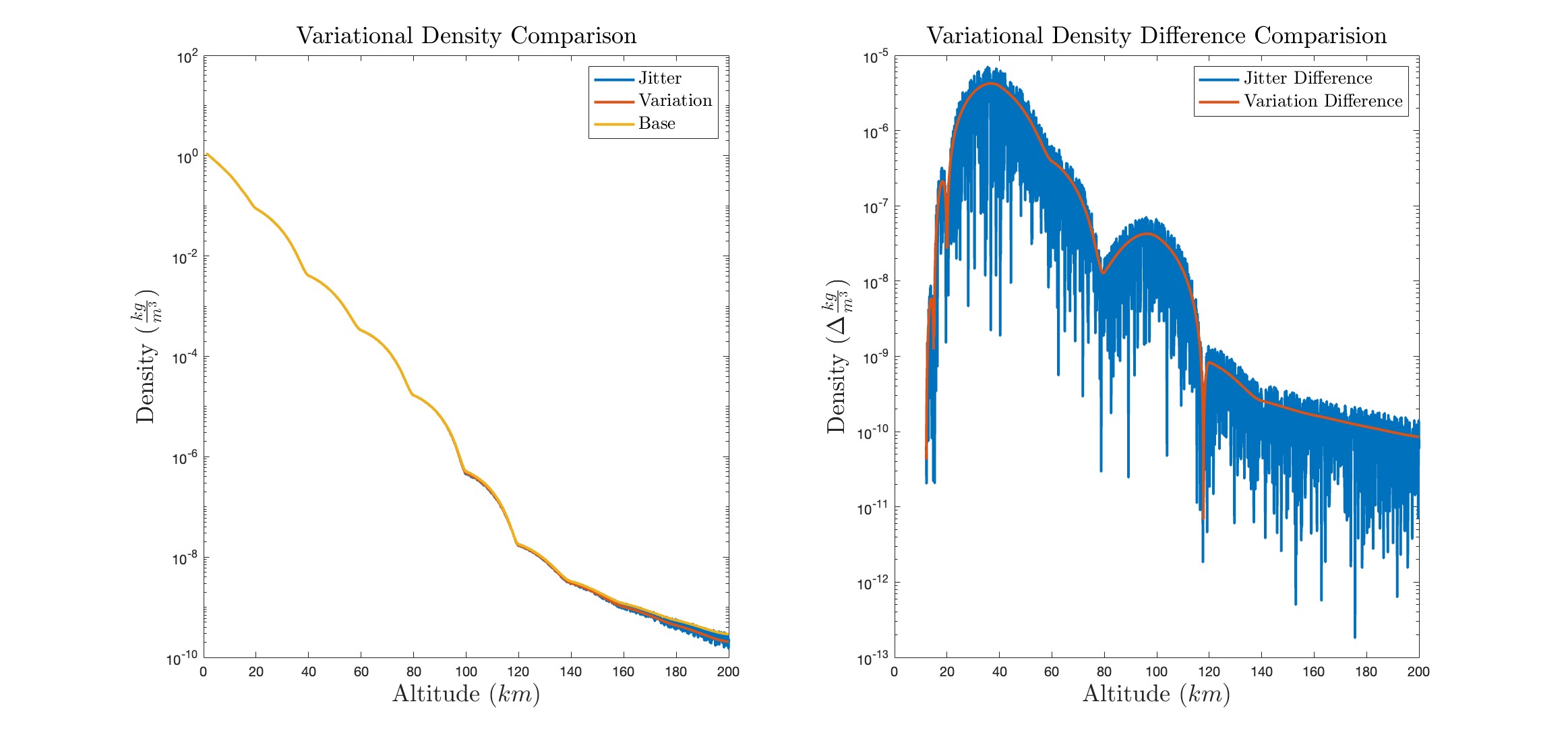
We consider drag using deterministic models that depend on a constant value, vary with altitude, vary with temperature and pressure, and probabilistic models that vary with a base offset value and a jittered offset, which includes a randomized base offset, that varies proportionally throughout the range of values, and a proportional randomized value that varies at each data point.
Trajectory Analysis
Staged Model
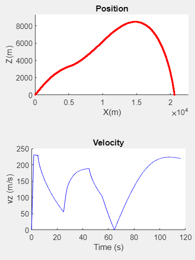
The ideal rocket qAs rockets expend fuel they not only lose mass, but they often eject the exhausted thrusters. We accounted for this loss by focusing on the stages of the rocket. As the rocket moves it loses mass as the fuel is expended, however upon the thrusters reaching the time in which the fuel is completely burnt (tburn) it will instantaneously eject and lose the remaining mass of the thruster. Our model accounts for changes in mass as well as thrust and staged values that can be expended as the rocket travels a trajectory. We focus on stages where fuel is 15% of the total mass, so that the rocket would have repeatable and observable changes in trajectory. The rocket modules expend mass continually at 15% intervals and until a total mass of 85% is ejected.
Model Application
As far as the scale of application of this project, the variation in the temperature, pressure, and density of the is a marginal effect in variation of the modeled drag coefficients. In the low atmosphere, less than 40km altitude, there is almost no variation in temperature due to solar activity. Specifically, solar temperature variation between 20km and 40km altitude contributes to a change of less than 1ºC. In these models, it would be more appropriate to study climatic, solar geometric factors of seasons, or other factors the would increase the magnitude of variation at low altitude.
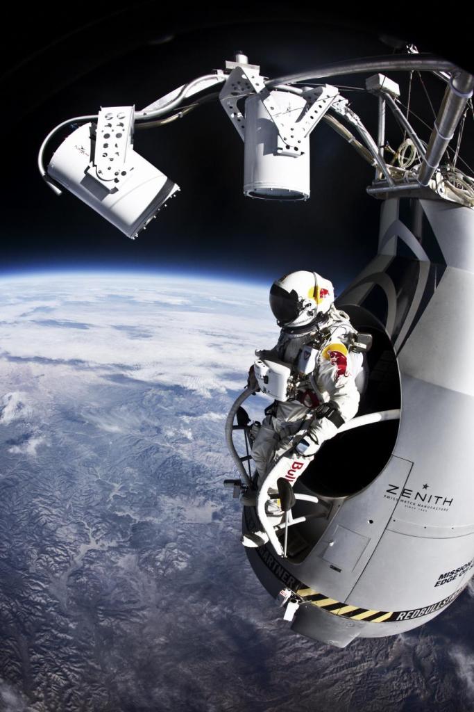
For reference, when Felix Baumgartner jumped out of an atmospheric ballon to set the record for the highest balloon flight, highest free fall, and the highest free fall velocity achieved by a person, he did so from just below 40km.3 Geosynchronous or Geostationary Orbits are around 36,000 km, Medium Earth Orbits are between 2,000-36,000 km, and Low Earth Orbits at the 2,000km altitude.4
If the objective of the model is to evaluate Missile and Rocket trajectories are planned in such a way so as to optimize the energy loss due to drag in periods of high drag.
These models can be expanded to consider the potential for payload delivery and separation of components in the rockets, such as releasing an expanded thruster.
Standard Drag Coefficient

ALTITUDE-BASED DRAG COEFFICIENT
Conclusion
Initial estimates of coefficients produced results that produced large differences between standard- and altitude based coefficients, range can vary as much as an order of magnitude at low altitudes and these differences grow
Variations in the models were minimized by adjusting coefficients and comparing trajectory features such as range and duration, peak, and stage transitions. Modeling using Standard- and Altitude-based drag showed nearly indistinguishable trajectory and drag at low, below 20km, atmosphere altitudes.
We are able to match the duration of five models within 100 steps for a 16,000-step Modified Euler.
Variations increased drastically at higher altitudes when variation temperature and density ranges increase. Additionally identify major characteristics, and the magnitude of these changes, in trajectories for similar conditions.
If we were to continue research we would consider approaches and models to evaluate climatic and seasonal temperature changes and radial gravity. We also plan to consider orbital mechanics or measuring the trajectory of separated modules.
Rocket Test
References
1 Bartholomew, A and Magnes, J. Computational Simulation of Rocket Trajectories from Modeling and Experimental Tools. 2019. https://pages.vassar.edu/magnes/2019/05/12/computational-simulation-of-rocket-trajectories/
2 Braeunig, Robert A. Basic of Space Flight: Atmospheric Models. 2014. http://www.braeunig.us/space/atmmodel.htm.
3 Crouch, T. The Big Jump. 2014 . https://ntrs.nasa.gov/api/citations/19780004170/downloads/19780004170.pdf
4 Brooks, D. An Introduction to Orbit Dynamics and its Application to Satellite-Based Earth Monitoring Missions. 1977. https://ntrs.nasa.gov/api/citations/19780004170/downloads/19780004170.pdf
