In this paper, we discuss the significance of Burgers’ equation, where we review the history of this partial differential equation, establishing understanding and setting motivation for a thorough analysis analytically and computationally, and comparing our coded results with other established methods. We approached solving Burgers’ equation by using the finite difference method, which we implemented in Python, identified analytic and computational solutions and obtain results consistent with the examples available in literature, including the Cole-Hopf transformation. Finally, we look into how Burgers’ equation is applied in fields not only related to physical research such as the simplification of Navier-Stokes equations and plasma flow, but beyond that, which include traffic flow, where it utilizes the one-dimensional Burgers’ equation.
Keiichi Iguchi, Andrew Liebig, and Calvin Puch
Department of Physics and Biophysics, Augusta University
(Dated: December 11, 2023)
Code Samples and some of the media from research are listed below
Interactive Graphs of Cole-Hopf Transforms available on Desmos
https://www.desmos.com/calculator/pztr22gzdo
https://www.desmos.com/calculator/aaciuaa5ta
import numpy as np
import sympy as sp

%matplotlib inline
from matplotlib import rcParams
rcParams['font.family'] = 'serif'
rcParams['font.size'] = 16

from sympy import init_printing
init_printing()
x, nu, t, a, b, k = sp.symbols('x nu t a b k')
## ensures that all variables used in computation is real

w = b + a*sp.exp(-nu*t*(k**2))*sp.cos(k*x)
wprime = a*k*sp.exp(-nu*t*(k**2))*sp.sin(k*x)
from sympy.utilities.lambdify import lambdify

u = -2*nu*(wprime/w)
ufunc = lambdify([t, x, nu, a, b, k], u, "numpy")
import matplotlib.pyplot as plt

nx = 101
nt = 100
dx = 2*np.pi/(nx-1)
nu = 0.07
dt = dx*nu
n = 1
x = np.linspace(0, 2*np.pi, nx)
un = np.empty(nx)

t=0
u = np.asarray([ufunc(t, x0, nu, 7.2, 15.22, 1.85) for x0 in x])
u = numpy.asarray([ufunc(t, x0, nu) for x0 in x])
import matplotlib.animation
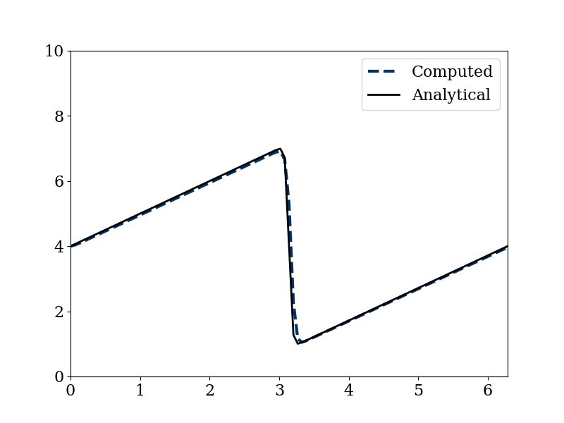
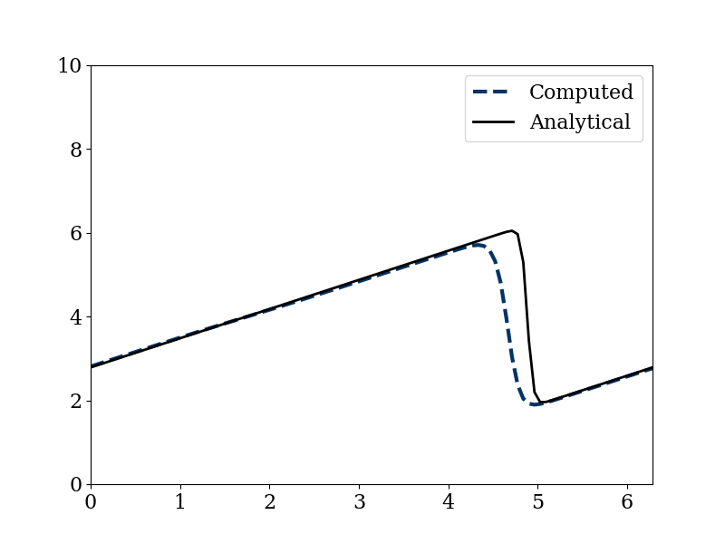
fig = plt.figure(figsize=(8,6))
ax = plt.axes(xlim=(0,2*np.pi), ylim=(-1,1))
line = ax.plot([], [], color='#003366', ls='--', lw=3)[0]
line2 = ax.plot([], [], 'k-', lw=2)[0]
ax.legend(['Computed','Analytical'])
def burgers(n):
un = u.copy()
u[1:-1] = un[1:-1] - un[1:-1] * dt/dx * (un[1:-1] - un[:-2]) + nu*dt/dx**2*\
(un[2:] - 2*un[1:-1] + un[:-2])
u[0] = un[0] - un[0] * dt/dx * (un[0] - un[-1]) + nu*dt/dx**2*\
(un[1] - 2*un[0] + un[-1])
u[-1] = un[-1] - un[-1] * dt/dx * (un[-1] - un[-2]) + nu*dt/dx**2*\
(un[0]- 2*un[-1] + un[-2])
u_analytical = np.asarray([ufunc(n*dt, xi, nu, 7, 15.22, 1.85) for xi in x])
line.set_data(x,u)
line2.set_data(x, u_analytical)
ani = matplotlib.animation.FuncAnimation(fig, burgers,
frames=nt, interval=100)
from IPython.display import HTML
HTML(ani.to_jshtml())